High Level Overview of the Signal Processing Pipeline of JAXPint (WIP)#
The PTA signal processing pipeline from raw TOA data to log likelihood evaluation is a bit confusing to an outsider. This is my best attempt at explaining this from end to end; this is also my mental model that I had in mind when building JAXPint.
For a visual summary of all of this:
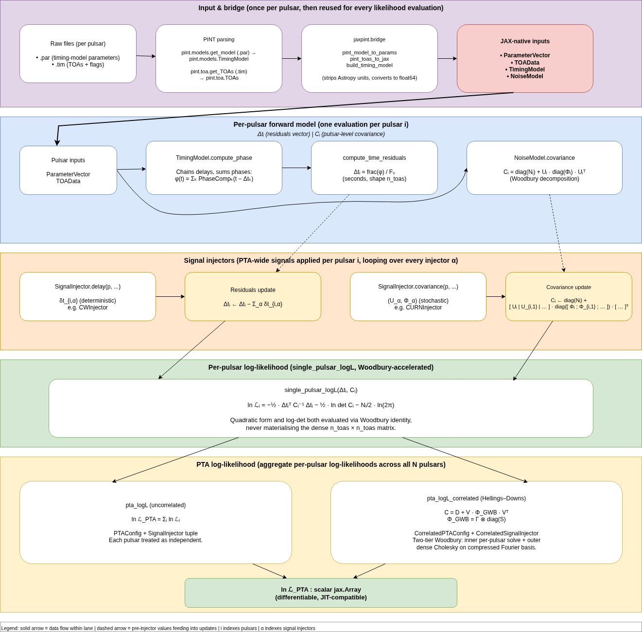
End-to-end flow: raw .par/.tim files → PINT parsing and JaxPINT bridge → per-pulsar forward model (residuals + covariance) → signal injector contributions → per-pulsar Gaussian log-likelihood → PTA log-likelihood (uncorrelated sum, or Hellings-Downs correlated).#
Input Data#
Each pulsar in the array is represented by two different files: a .par file and .tim file
.tim File#
The .tim file is a list of one time-of-arrival (TOA) per line, plus a handful of optional file-level directives. JaxPINT reads these via PINT, so anything PINT understands works here. Since PTAs have been around for a while, there are a smorgasbord of different formats.
For simplicity, let’s just look at one of these formats: TEMPO2 format. The first line must be FORMAT 1, and every subsequent TOA line has five positional fields followed by zero or more -flag value metadata pairs:
name freq_MHz MJD uncertainty_us site [-flag value]*
Example:
.tim file (TEMPO2 format)#FORMAT 1
J1834-0701_L.guppi.1 1500.000 58423.5001352123456 0.312 gbt -be GUPPI -fe Rcvr1_2 -pta NANOGrav
J1834-0701_L.guppi.2 1500.000 58423.5001352123456 0.298 gbt -be GUPPI -fe Rcvr1_2 -pta NANOGrav
J1834-0701_S.guppi.1 2100.000 58424.7614293182746 0.405 gbt -be GUPPI -fe Rcvr2_3 -pta NANOGrav
The trailing -flag value pairs are free-form metadata attached to each TOA. PTAs use them to tag the backend, frontend, observing group, receiver, etc. JaxPINT’s noise model selects per-TOA EFAC, EQUAD, and ECORR values by matching against these flags, so the same flag keys have to appear consistently in the .tim file and the .par file.
TEMPO2 also defines a small set of in-file commands (TIME offsets, EFAC, EQUAD, MODE, SKIP/NOSKIP, INCLUDE, JUMP/NOJUMP) that PINT applies on read. Unlike the .par parameter set, there is no single enumerated catalog of flag names – each PTA defines its own conventions. See the TEMPO2 manual for the authoritative format specification, and the PINT explanation page for PINT-specific notes on what happens when the file is loaded.
Some important observations#
The fundamental unit of data for a TOA is the triple
consisting of the observing frequency \(\nu\) (MHz), the pulse arrival time \(t\) (MJD), and the measurement uncertainty \(\sigma_t\) (µs). Everything else is metadata which is either documentation, or flags which alter one of these values
Each frequency gets assigned its own TOA, even if they were observed at the same MJD.
There is no gaurentee on uniform cadence between TOAs (which makes sense, since the telescope could be down for maintainance or someething)
Parsing .tim files in JAXPint#
I made the pragmatic decision to offload the TOA parsing to PINT. I didn’t want to deal with all the nuances of different time standards, flags and backends and probably other things that I’m forgetting.
The .tim parsing workflow is the read in .tim files via PINT, which results in a pint.toa.TOAs object (an astropy.table.Table with one row per TOA) – and then converted that into a JAX-compatible container, TOAData, via pint_toas_to_jax().
In principle, it would be straightforward to skip the PINT parsing dependency and just write directly to TOAData.
.par File#
This is just a plain table of values which specifies how to build a particular pulsar model.
.par file#PSR J1834-0701_00
RAJ 18:34:29.80260
DECJ -07:01:17.6778
F0 443.4391679646
F1 -2.481624e-15
PEPOCH 57000.0
DM 49.0249
PX 1.359724
EPHEM DE440
CLK TT(BIPM2019)
UNITS TDB
EFAC tel gbt 1.0
EQUAD tel gbt 0.1
Most of the parameters in PINT are supported (with the exception of some obscure stuff). See the PINT supported parameters table for the full list of accepted keywords, units, and aliases.
Parsing .par files in JAXPint#
JAXPint currently outsources the initial parsing and construction of the pulsar timing model to PINT. This was done for reasons exactly analagous to PINT. I don’t want to be writing parsers that have already been written.
The flow mirrors the .tim case:
The raw
.parfile is read by pint.models.get_model, which returns a pint.models.TimingModel object. That object holds every parameter as anastropy.units.Quantityand tracks PINT’s component hierarchy (delays, phases, noise).The PINT
TimingModelis then handed to the JaxPINT bridge layer, which produces two JAX-native objects:pint_model_to_params()extracts every numerical parameter into a flatParameterVector– the only differentiable leaf of the pytree.build_timing_model()constructs the JAX-nativeTimingModel. Astropy units are stripped and every scalar becomes plainfloat64.
Once this conversion is done, the PINT object is no longer needed at runtime – the rest of the pipeline operates entirely on the JaxPINT types.
Synthetic Versus Real Data#
As an aside, notice that the pipeline doesn’t care about the origin of the .par and .tim files. Hence, you could run JAXPint on real pulsar data, or you can generate synthetic .par and .tim files.
For synthetic data generation, you could use PINT’s model construction facilities, generate a uniform time series of observations with pint.simulation.make_fake_toas_uniform (or one of the other generators in pint.simulation), and then pass the two through the pipeline to get the JAX-compatible model and time data.
If you have some external signal (re: CW gravitational wave of a stochastic GW background), you could also generate a mock timeseries to reflect these injected signals.
TimingModel#
TimingModel is the deterministic side of the pipeline, and it is best thought of as a forward model: given a ParameterVector and a TOAData, it predicts a pulsar rotational phase for each TOA. The output has the same shape as the input timestamps – (n_toas,) – but the values are phases (cycles), not modified times.
Every TOA marks a moment where the pulse beam swept past Earth, so by construction the observed phase is always a pulse peak – i.e. integer phase, modulo one cycle. TimingModel predicts what phase the pulsar should have been at at that same moment. If the prediction lands at e.g. \(12{,}345{,}678{,}901.2346\) cycles, the integer portion tells us which pulse we caught and the fractional \(0.2346\) tells us how many cycles off the model was from reality. Dividing that sub-cycle mismatch by \(F_0\) converts it into the time residual the fitter actually minimises.
Internally, TimingModel holds three tuples of components – delays, phases, and dispersion – and combines them in different ways.
Delay components#
A “delay” here is the correction between the topocentric TOA (what the telescope recorded, after PINT’s clock corrections) and the time at which the pulsar’s intrinsic spin model – the \(F_0, F_1, \ldots\) polynomial – actually applies. That reference time is effectively the pulse emission time in the pulsar’s rest frame. Concretely, if \(t\) is the topocentric TOA and \(\Delta t_\mathrm{total}(t)\) is the full delay, the phase model is evaluated at
Each individual \(\Delta t_k\) accounts for one physical reason the pulse took longer to reach the telescope than the pulsar’s own clock would suggest:
Component |
Correcting for |
|---|---|
Astrometry (Rømer) – |
Light-travel time between the solar-system barycenter (SSB) and the observatory – i.e. Earth’s position in its orbit. Biggest term, up to ~500 s. |
Shapiro (solar system) – |
Gravitational time dilation as the pulse passes near the Sun. |
Dispersion (ISM) – |
Frequency-dependent slowdown from free electrons along the line of sight. |
Troposphere – |
Signal slowdown through Earth’s atmosphere. |
Binary (Rømer / Einstein / Shapiro) – |
For binary pulsars: light-travel, gravitational redshift, and Shapiro delay inside the pulsar’s own orbit. |
Walking the delay_components tuple in order effectively steps the reference frame outward along the signal path: observatory → SSB → pulsar system barycenter → pulsar surface.
The accumulating chain#
compute_delay() walks the delay_components tuple sequentially. Each component contributes an additive term, but sees the accumulated delay from prior components as an input. The final value is still a simple sum,
where
\(t\) is the topocentric TOA (the observation time read from the
.timfile, after clock corrections).\(k\) indexes the entries of the
delay_componentstuple, walked in order.\(\Delta t_k(\cdot)\) is the delay contribution produced by the \(k\)-th component, in seconds. Each component is a callable that takes the TOA data and the accumulated delay so far.
\(\Delta t_{<k} \equiv \sum_{j<k} \Delta t_j\) is the running sum of all component contributions before \(k\). Passing this in as the second argument is what lets later components (e.g. binary orbital delays) operate in the frame the earlier components have already corrected for.
\(\Delta t_\mathrm{total}(t)\) is the final summed delay at \(t\), returned by
compute_delay().
The order matters because \(\Delta t_k\) is in general a function of \(\Delta t_{<k}\), not just an additive constant. A binary-orbit Rømer delay, for instance, has to be computed in the SSB frame – which only exists once the astrometric correction has already been peeled off. If two components genuinely commute (their contributions don’t depend on prior delay), their ordering is irrelevant; in practice most components are weakly order-dependent.
Phase components#
compute_phase() sums the contributions from every component in phase_components. Addition is commutative, so order is irrelevant here. Each component receives the total delay from above as input, then returns its own phase contribution as a DualFloat (an integer + fractional cycle split, kept separate to preserve double-precision over long baselines).
Some examples of phase components:
Component |
What it contributes |
|---|---|
The bulk of the phase: a Taylor expansion \(\varphi(t) = F_0 \Delta t + \tfrac{1}{2} F_1 \Delta t^2 + \ldots\) around the reference epoch |
|
Discrete spin-up events: a step in \(F_0\) (and optionally \(F_1\)) at a specified epoch, occasionally with an exponentially decaying recovery term. |
|
Arbitrary additive phase offsets applied to subsets of TOAs selected by |
After summing, the model subtracts the phase at the TZR reference TOA to get absolute phase, then applies the PHOFF offset if present.
When this absolute phase is fed into compute_phase_residuals(), the integer portion is reconciled against delta_pulse_number (which pins each TOA to a specific integer pulse). Only the fractional part survives as the residual – the integer pulse count cancels out, leaving the sub-cycle timing mismatch that the fitter tries to minimise.
Dispersion components#
Dispersion components are a specialisation (DispersionDelayComponent) that participate twice:
In the delay chain. Every dispersion component is also a delay component, so its timing contribution is folded into the sequential
compute_delaychain described above.In a separate DM sum.
compute_dm()sums each component’s \(\mathrm{DM}\) contribution across thedispersion_componentstuple to produce a per-TOA DM (in pc/cm³). This is used by the wideband fitter (WidebandGLSFitter) to form DM residuals alongside the time residuals.
For narrowband fits, only the first role matters; compute_dm is simply not called.
NoiseModel#
NoiseModel is the stochastic side. Every correlated noise source contributes a block to a single, unified pulsar-level covariance matrix expressed in Woodbury form:
\(N_\mathrm{diag}\) comes from the white-noise component (
ScaleToaErrorapplyingEFAC/EQUAD). When absent, the raw TOA uncertainties are used.\(U\) is the horizontal concatenation of the basis matrices from every correlated component (
ECORR, red noise, DM noise, chromatic noise, …).\(\Phi_\mathrm{diag}\) is the concatenation of the corresponding per-basis weights.
Each individual noise component contributes linearly. Adding a new noise source means appending a few columns to \(U\) and a few entries to \(\Phi_\mathrm{diag}\), nothing else.
covariance() returns the triple \((N_\mathrm{diag},\; U,\; \Phi_\mathrm{diag})\), which the GLS fitters then feed directly into the Woodbury identity to avoid ever materialising the dense \(n_\mathrm{toas} \times n_\mathrm{toas}\) covariance.
Fitting#
Once the raw .par/.tim files have been converted to JAX-native objects, everything downstream is pure JAX code – no more Astropy units, no more PINT dependency at runtime. A fit takes four inputs:
TimingModel– the deterministic timing model (chained delays + summed phases).TOAData– observation times, frequencies, uncertainties, SSB positions, etc.ParameterVector– current parameter values, plus a frozen/free mask that determines which parameters actually move.NoiseModel– optional; carriesEFAC/EQUAD/ECORR/red-noise contributions.
Residuals#
Residuals come in two flavors, both pure functions of (model, toa_data, params):
compute_phase_residuals()returns the fractional part of the model phase (in cycles), withdelta_pulse_numberoffsets accounted for.compute_time_residuals()wraps the phase residuals and divides by the spin frequency \(F_0\) to return residuals in seconds.
Both return a jax.Array of shape (n_toas,).
PTA Likelihood Construction#
All of the above holds on a per pulsar level. For PTA, you run this procedure for each pulsar timeseries in your PTA to generate a set of time-residuals (ie. What offset do you need to apply to the given MJDs which best matches the given pulsar model?).
Denote the i-th pulsar timing residual as \(\Delta t_i\) and its pulsar-level covariance (built by the NoiseModel) as \(C_i\). The number of toas per pulsar is denoted as \(N_{i}\).
Per-pulsar Gaussian log-likelihood#
Under the usual assumption that each pulsar’s residuals are a zero-mean Gaussian with covariance \(C_i\), the per pulsar log-likelihood is
Because \(C_i\) has the Woodbury structure \(C_i = \mathrm{diag}(N_i) + U_i\,\mathrm{diag}(\Phi_i)\,U_i^{\mathsf{T}}\) (see the NoiseModel section), both the quadratic form and the log-determinant can be evaluated in \(\mathcal{O}(n_\mathrm{toas}\,n_\mathrm{basis}^2)\) time without ever materialising the dense \(n_\mathrm{toas}\times n_\mathrm{toas}\) matrix.
Putting it together#
A minimal end-to-end PTA log-likelihood evaluation:
from jaxpint.pta.likelihood import PTAConfig, pta_logL
from jaxpint.pta.params import GlobalParams
from jaxpint.pta.signals.cw import CWInjector

# one entry per pulsar (from the bridge layer)
toa_data_list  = (toa1, toa2, toa3)
timing_models  = (tm1,  tm2,  tm3)
noise_models   = (nm1,  nm2,  nm3)
pulsar_params  = (p1,   p2,   p3)

injectors = (CWInjector(...),)                         # deterministic CW
config    = PTAConfig(toa_data_list, timing_models,
                      noise_models, injectors)
global_params = GlobalParams.empty()
for inj in injectors:
    global_params = inj.register_params(global_params)

logL = pta_logL(global_params, pulsar_params, config)  # scalar jax.Array
Swapping pta_logL for pta_logL_correlated() (with a CorrelatedPTAConfig and one or more correlated injectors) turns on the Hellings-Downs coupling. Because both functions are pure JAX, the whole thing plays nicely with jax.jit, jax.grad, and downstream samplers like BlackJAX.